In this tutorial, you will learn how to get currency data into Excel using different methods.

Introduction
Excel spreadsheets are a powerful tool with countless usages possibilities. With its many possibilities however one can easily feel overwhelmed. When it comes to currency exchange rates, Excel 365 enables you to work with them in the program. The feature, however, is not easy to find at first glance since it is part of the stocks‘ data feed.
So, if you are looking to compare different currencies in Excel, we have got you covered. In this article, you will learn how to enter currency data into Excel, how to compare currency pairs, convert them to a data type, how you create a currency conversion calculator, and how to extract the information.
The scope of this task will differ, depending on how many currencies you want to compare. Generally, there are two levels of getting currency data into Excel:
- Comparing multiple currencies with daily updated rates : this can be done with the help of the data stocks feature, which supports 160 worldwide currencies.
- Comparing multiple currency values with up-to-date conversion rates : this is more advanced and extensive, but also more accurate with a higher number of currencies.
Getting Started with currency data in Excel 365
- Open a new Excel sheet
- Enter a currency pair in a cell. Keep in mind you must use this format: "From Currency to currency" with the ISO currency codes. You can separate the two currencies by a space, dash, colon, or slash. The first currency hereby is the one that is buying the second.
For example: "USD/EUR" will get you the exchange rate from 1 US Dollar to Euros. “GBP-CAD” will get you the exchange rate from 1 UK Sterling to Canadian Dollars.
Method 1: Comparing Currencies in Excel
Once you have your cells in the right format, Excel 365 offers a feature called "Stocks". This allows you to work with daily updated currency exchange rates.
Here is how you proceed:
-
To make the process easier later, we advise you to create a table first. This step is not mandatory but will be helpful later. To do so, select the cells and click on Insert > Table.
-
Select the correctly formatted cells that you want to convert.
-
Open the Data tab and click on "Stocks"
-
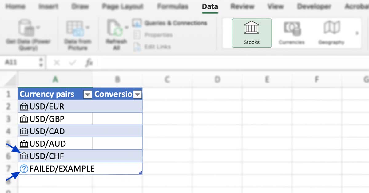
If Excel finds a match for your currency pairs, it converts them into a data type. If your format is correct, and data is found, the stock icon will appear in your cells.
-
If you see the question mark symbol in your cells, something went wrong (see our example below). This could be due to the wrong format, or not using the standardized designation for a currency. Simply correct any mistakes and press enter to try again.
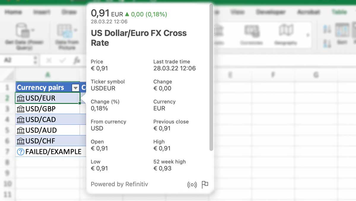
- Now that you have converted the cells you can extract more information from them by clicking the stock icon. A card will pop up, that shows you information about the relationship between the two currencies.
- Now that you have converted the cells you can extract more information from them by clicking the stock icon. A card will pop up, that shows you information about the relationship between the two currencies.
Other ways to show the card are:
- Clicking the icon on the left of the main data cell
- Right-click on the data and choosing "show card".
- Shortcut: CTRL (for Mac CMD) + Shift+F5
The information from the pop-up card can also be shown in columns. To do so you can click the "insert data" button.
This can be done by clicking the Insert Data icon that appears in the pop-up card next to a category or if you close the pop-up it is visible next to the table.
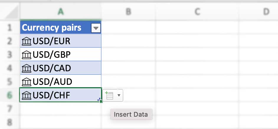 If you close the pop-up and click the symbol next to the table, it opens a list of all the fields available. By clicking a field, a new column is automatically created.
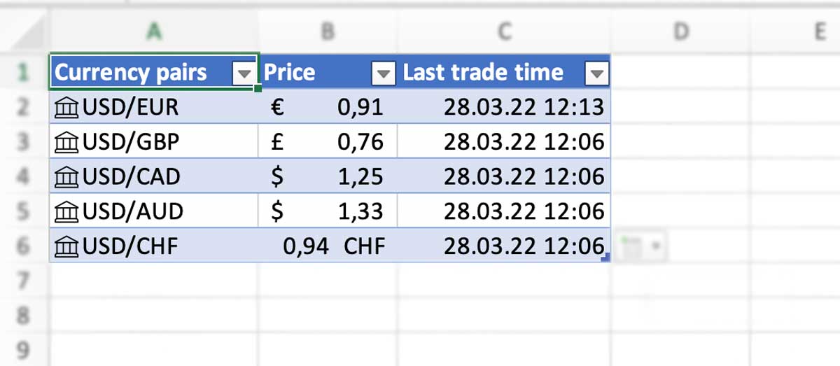
For example, Price will show you the exchange rate for the currency pair. If your cell says EUR/USD, the price column will tell you how much one Euro is in US Dollar. The Last Trade Time option tells you, at what time the rate was quoted.
- Another way to get your information is by using a formula. To do so, reference the cell you want to calculate and then press dot and select or enter the category you are looking for and then hit your enter key.
For example, we type "=", then select the cell "EUR/USD" and then chose the category "price".
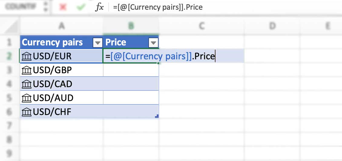
This will create a new column that shows the prices for all the currency pairs.
So, the formula in our case is: =A2.price
- Now that you have all the necessary currency data, you can use it in your calculations and formulas.
- The data will of course not update itself automatically. To ensure your data is up to date, you can refresh it manually under Data > Refresh all.
Method 2: Live currency rates in Excel
Since Excel only provides as-is information we now look at what to do if you want or need to work with live currency rates in Excel.
We have prepared a step-by-step guide on how to import and update live exchange rates via an API in Excel. You won´t need any programming skills to follow this tutorial.
Get a currency API
The most common and accurate way to get live currency rates in Excel is by using an API. We are using CurrencyAPI.com, as it offers over 170 currency pairs and updates its data up to every 60 seconds. You can find the documentation here. It also offers a free version in case you want to try it out first.
Live currency rates in Excel
To get started, open a spreadsheet and sign into your API.
Step 1: Create a Web Query
The first step is creating the web query to fetch the exchange rates. To do that go to the Data Tab and click on "from Web".
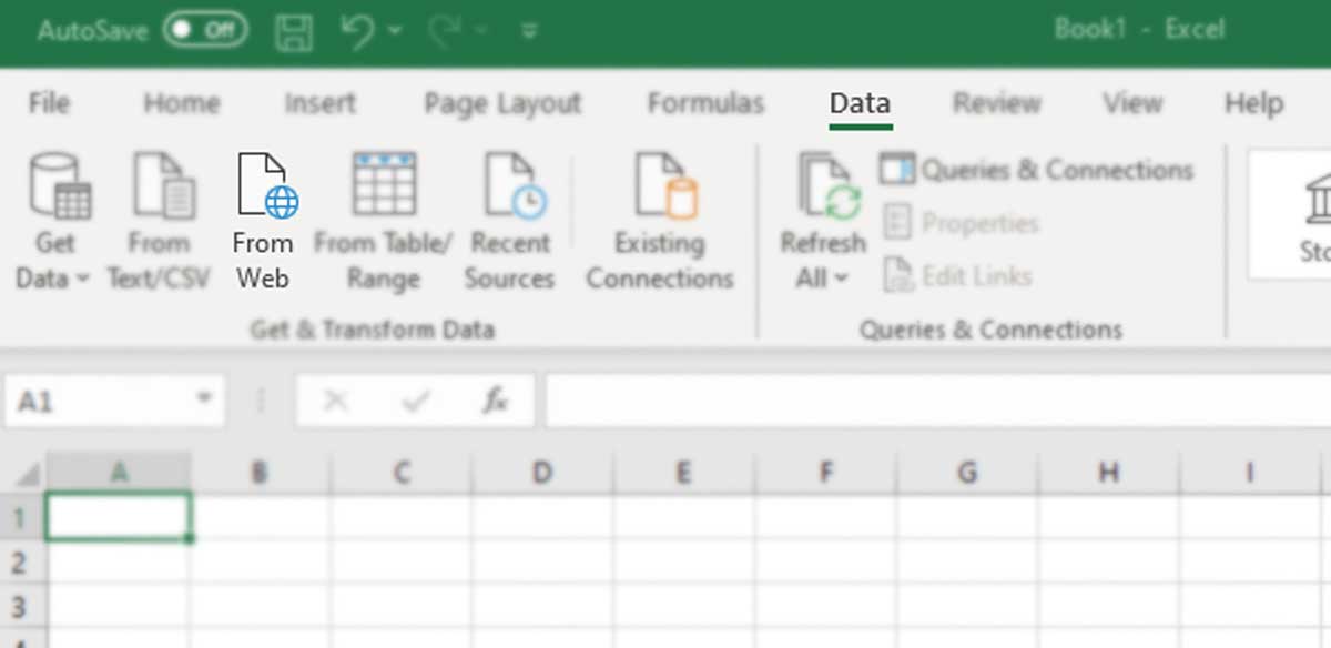
A window appears that asks for an URL. Enter the query with your own unique API key:
The base currency here automatically is USD.
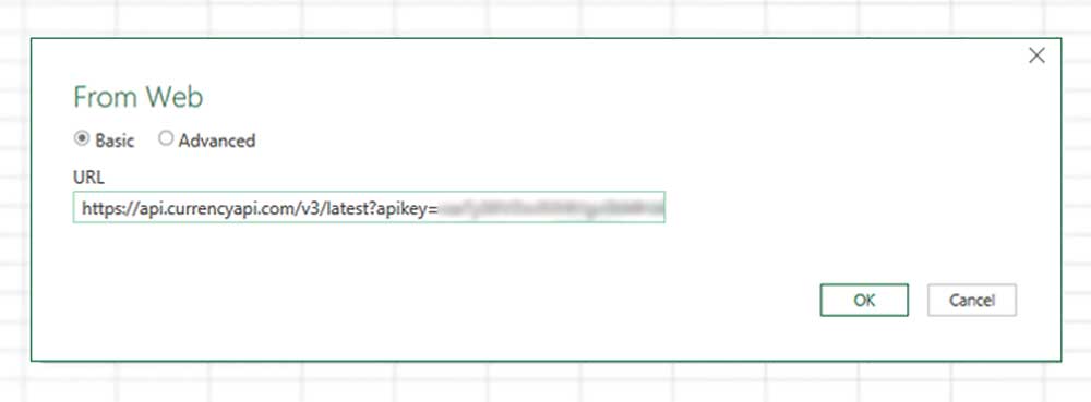
After that click OK.
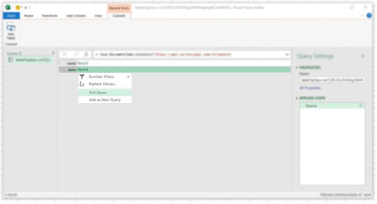
Step 2: Drill Down
Once we click on OK, we get directed to another box. Right-click on Record next to Data and then select “Drill Down”.
Step 3: Into table
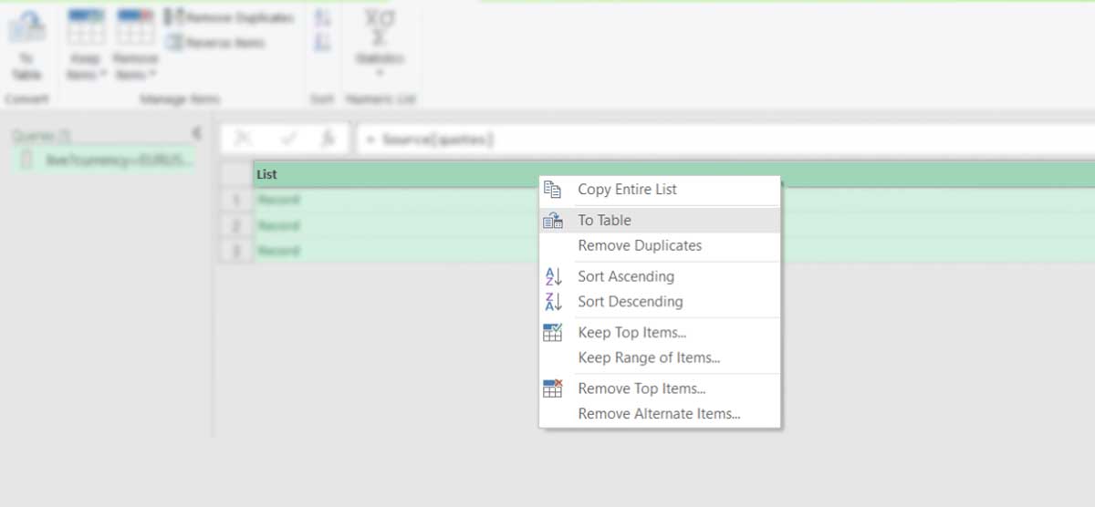
Clicking on Drill Down will redirect us again. We now right-click on the first conversion and select ”Into table“. Click OK on the Window that appears after this.
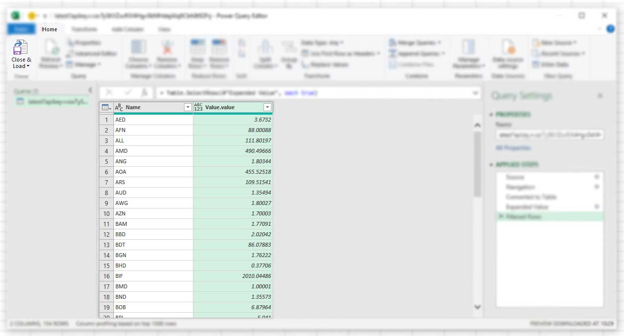
Step 4: Close and load
Now we have the live rates in the boxes. Click on Close & Load in the left upper corner.
And that's it!
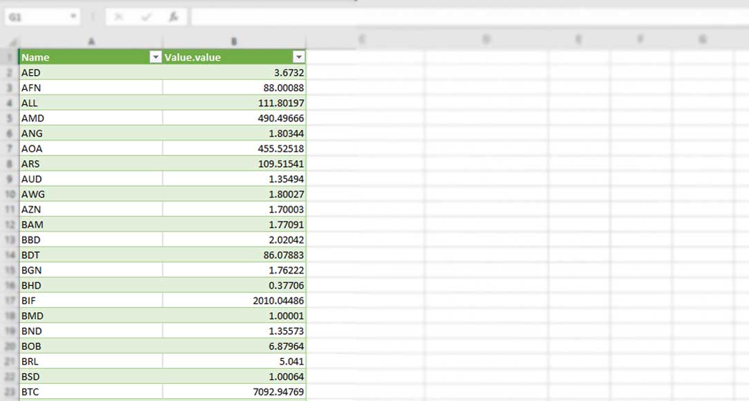
We now have the live currency exchange rates in our Excel Sheet. If you want to work with the latest prices, simply click on Table Design > Refresh.